import bindcurve as bc
import pandas as pd
import matplotlib.pyplot as pltBasics of BindCurve
In this tutorial, we will go through the very basics of bindcurve. We will fit \(\text{IC}_{50}\) for six compounds and plot the results. This will demonstrate the most minimalistic workflow you can do to get your results quickly and easily. For clarity, we will mostly use default settings for all the bindcurve functions. There is much more you can do, please see more advanced tutorials for more detailed overview of the available options and settings.
Preparations
First, let’s start by importing bindcurve. We will use bc as alias to help with clarity. Also, we will import pandas and matplotlib because we will need it. Don’t worry, all dependencies have been installed automatically when installing bindcurve.
The following settings adjust the decimals and display width for pandas. This is just for display purposes, all numbers will still be stored with many decimal places.
pd.set_option("display.precision", 2)
pd.set_option('display.width', 200)
Load the data
With all preparations taken care of, let’s load our data from csv file using the load_csv function. You can find this data on GitHub in the folder /tutorials/examples/competitive.csv. We will load the data into a DataFrame which we will call input_data. As you can see, the loaded data have been preprocessed and now newly contain log-transformed concentrations (log c) as well as number of replicates (n_reps) and median response values with SD snd SEM metrics for each concentration point. This has all been added by the load_csv function, so that the loaded DataFrame contains all the necessary information for further use in bindcurve.
input_data = bc.load_csv("examples/competitive.csv")

print(input_data)
Loading data from examples/competitive.csv
compound c log c n_reps r1 r2 r3 r4 r5 r6 median SD SEM
0 comp1 2000.00 3.30 6 28 26 29 27 27 25 27.0 1.41 0.58
1 comp1 1000.00 3.00 6 30 28 30 28 32 32 30.0 1.79 0.73
2 comp1 250.00 2.40 6 37 40 37 41 42 38 39.0 2.14 0.87
3 comp1 60.00 1.78 6 60 58 54 58 53 57 57.5 2.66 1.09
4 comp1 15.00 1.18 6 82 84 78 85 84 85 84.0 2.68 1.10
5 comp1 4.00 0.60 6 94 88 91 97 95 100 94.5 4.26 1.74
6 comp1 1.00 0.00 6 97 98 96 102 103 106 100.0 3.93 1.61
7 comp1 0.25 -0.60 6 100 100 101 106 106 108 103.5 3.56 1.45
8 comp1 0.06 -1.22 6 100 101 102 97 109 109 101.5 4.94 2.02
9 comp2 2000.00 3.30 6 27 29 31 26 27 30 28.0 1.97 0.80
10 comp2 1000.00 3.00 6 24 28 26 25 29 30 27.0 2.37 0.97
11 comp2 250.00 2.40 6 32 33 30 28 30 30 30.0 1.76 0.72
12 comp2 60.00 1.78 6 31 33 39 38 41 34 36.0 3.90 1.59
13 comp2 15.00 1.18 6 53 55 61 62 53 57 56.0 3.92 1.60
14 comp2 4.00 0.60 6 82 78 82 75 86 87 82.0 4.59 1.87
15 comp2 1.00 0.00 6 91 88 86 96 97 100 93.5 5.51 2.25
16 comp2 0.25 -0.60 6 97 99 95 102 100 100 99.5 2.48 1.01
17 comp2 0.06 -1.22 6 100 98 94 105 102 109 101.0 5.28 2.16
18 comp3 2000.00 3.30 6 25 25 20 24 22 20 23.0 2.34 0.95
19 comp3 1000.00 3.00 6 24 26 23 25 26 21 24.5 1.94 0.79
20 comp3 250.00 2.40 6 21 26 25 25 25 24 25.0 1.75 0.71
21 comp3 60.00 1.78 6 27 27 30 27 24 29 27.0 2.07 0.84
22 comp3 15.00 1.18 6 31 34 35 33 36 37 34.5 2.16 0.88
23 comp3 4.00 0.60 6 49 47 44 54 58 60 51.5 6.36 2.59
24 comp3 1.00 0.00 6 71 78 75 80 86 84 79.0 5.59 2.28
25 comp3 0.25 -0.60 6 84 91 87 98 97 102 94.0 6.97 2.85
26 comp3 0.06 -1.22 6 97 98 101 107 111 103 102.0 5.38 2.20
27 comp4 2000.00 3.30 6 25 24 22 22 23 25 23.5 1.38 0.56
28 comp4 1000.00 3.00 6 26 25 24 22 23 27 24.5 1.87 0.76
29 comp4 250.00 2.40 6 27 29 25 25 21 25 25.0 2.66 1.09
30 comp4 60.00 1.78 6 27 24 29 35 30 33 29.5 3.98 1.63
31 comp4 15.00 1.18 6 34 38 40 48 43 51 41.5 6.35 2.59
32 comp4 4.00 0.60 6 53 54 59 67 63 65 61.0 5.81 2.37
33 comp4 1.00 0.00 6 85 88 86 95 93 99 90.5 5.55 2.27
34 comp4 0.25 -0.60 6 98 93 96 105 105 105 101.5 5.35 2.19
35 comp4 0.06 -1.22 6 100 97 102 104 106 106 103.0 3.56 1.45
36 comp5 2000.00 3.30 6 25 26 32 26 27 27 26.5 2.48 1.01
37 comp5 1000.00 3.00 6 26 27 33 27 21 33 27.0 4.58 1.87
38 comp5 250.00 2.40 6 30 32 32 40 33 40 32.5 4.37 1.78
39 comp5 60.00 1.78 6 52 50 48 54 50 57 51.0 3.25 1.33
40 comp5 15.00 1.18 6 73 77 77 78 80 79 77.5 2.42 0.99
41 comp5 4.00 0.60 6 92 90 88 91 96 100 91.5 4.40 1.80
42 comp5 1.00 0.00 6 92 92 91 104 104 101 96.5 6.31 2.58
43 comp5 0.25 -0.60 6 94 99 96 100 107 105 99.5 5.04 2.06
44 comp5 0.06 -1.22 6 95 96 99 102 109 108 100.5 5.96 2.43
45 comp6 2000.00 3.30 6 22 23 24 24 21 25 23.5 1.47 0.60
46 comp6 1000.00 3.00 6 23 24 25 24 20 27 24.0 2.32 0.95
47 comp6 250.00 2.40 6 26 27 33 27 21 33 27.0 4.58 1.87
48 comp6 60.00 1.78 6 30 32 32 40 33 40 32.5 4.37 1.78
49 comp6 15.00 1.18 6 52 50 48 54 50 57 51.0 3.25 1.33
50 comp6 4.00 0.60 6 73 77 77 78 80 79 77.5 2.42 0.99
51 comp6 1.00 0.00 6 92 90 88 91 96 98 91.5 3.78 1.54
52 comp6 0.25 -0.60 6 95 94 94 104 104 101 98.0 4.89 1.99
53 comp6 0.06 -1.22 6 94 99 96 100 107 105 99.5 5.04 2.06We can get the list of compounds available in our data and print the number of them.
compounds = input_data["compound"].unique()
print("Detected compounds:", compounds)
print("No. of detected compounds:", len(compounds))
Detected compounds: ['comp1' 'comp2' 'comp3' 'comp4' 'comp5' 'comp6']
No. of detected compounds: 6Fitting the model
Finally, we can fit a logistic model into our data. We will do that by using the fit_50 function and we will pass the input_data DataFrame and the model name as the arguments for this function. The function will output a new Dataframe containing the results, let’s call it IC50_results. The results contain the following information:
n_points: number of datapoints that were used for fittingIC50: value of \(\text{IC}_{50}\)loCL: lower confidence limit of the 95% confidence intervalupCL: upper confidence limit of the 95% confidence intervalSE: standard errormodel: name of the model that was usedymin: lower asymptote of the modelymax: upper asymptote of the modelslope: slope of the modelChi^2: estimate of \(\chi^2\) (the lower the better)R^2: estimate of \(R^2\) (the closer to 1 the better)
IC50_results = bc.fit_50(input_data, model="IC50")
print(IC50_results)
Fitting IC50 ...
compound n_points IC50 loCL upCL SE model ymin ymax slope Chi^2 R^2
0 comp1 54 41.89 35.65 49.82 3.37 IC50 25.45 103.37 -0.91 522.48 0.99
1 comp2 54 10.28 8.74 12.06 0.80 IC50 27.32 100.41 -1.06 693.80 0.99
2 comp3 54 2.13 1.67 2.63 0.23 IC50 23.30 104.77 -0.93 894.91 0.98
3 comp4 54 3.77 3.11 4.55 0.36 IC50 24.42 104.83 -1.02 1024.47 0.98
4 comp5 54 32.47 26.70 39.81 3.15 IC50 25.76 100.77 -1.00 929.11 0.98
5 comp6 54 8.97 7.62 10.54 0.71 IC50 23.52 100.92 -0.97 663.17 0.99We can also get the results as a formatted report using the report function. This will provide a convenient report in two formats:
- mean (95% confidence interval)
- mean ± SE
The last line will copy the report into your clipboard, you can then paste the results by CTRL+V anywhere you want.
IC50_report = bc.report(IC50_results, decimals=1)
print(IC50_report)
IC50_report.to_clipboard(excel=True, sep=",")
compound Mean (95% CI) Mean ± SE
0 comp1 41.9 (35.7, 49.8) 41.9 ± 3.4
1 comp2 10.3 (8.7, 12.1) 10.3 ± 0.8
2 comp3 2.1 (1.7, 2.6) 2.1 ± 0.2
3 comp4 3.8 (3.1, 4.5) 3.8 ± 0.4
4 comp5 32.5 (26.7, 39.8) 32.5 ± 3.1
5 comp6 9.0 (7.6, 10.5) 9.0 ± 0.7Plotting the curves
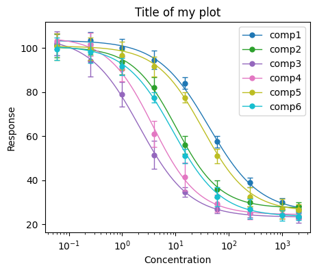
Plotting is done using the matplotlib library. We will initiate the plot in a standard way, then we will use the plot function, which will retrieve the curve from the model and draws it into the initiated plot. The required arguments for the plot function are the DataFrame with the input data (that is used to retrieve the concentration points), and the DataFrame with the results (that is used to draw the curve). Then we can use any common matplotlib settings, here we will set up title, axis labels, and set x axis to log scale. This way you have a lot of flexibility in designing your plot.
plt.figure(figsize=(5, 4))

bc.plot(input_data, IC50_results)

plt.title("Title of my plot")
plt.xlabel("Concentration")
plt.ylabel("Response")
plt.xscale("log")
plt.legend()

# Uncomment the below line if you want to save your plot as png
#plt.savefig("my_plot.png", dpi=300)

plt.show()
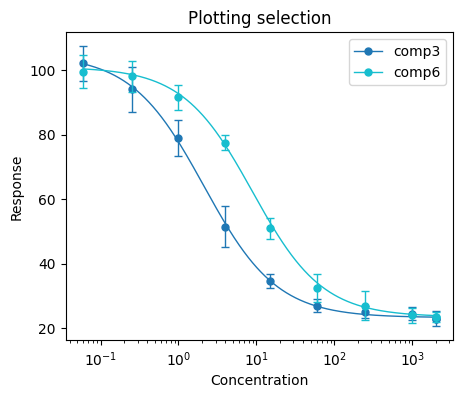
We can also plot just a selected compounds using the compound_sel argument. The selection is supplied as a list of compound names. In the following example, we will plot just the comp3 and com6 compounds.
plt.figure(figsize=(5, 4))

bc.plot(input_data, IC50_results, compound_sel=["comp3", "comp6"])

plt.title("Plotting selection")
plt.xlabel("Concentration")
plt.ylabel("Response")
plt.xscale("log")
plt.legend()
plt.show()
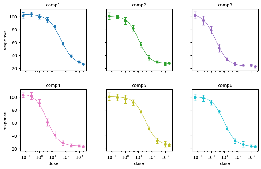
Finally, you can also plot the compounds on a grid using the plot_grid function. To do this, you don’t initiate the matplotlib plot in advance as in the case of the plot function. Instead, everything is executed by a single line of code. You have to supply all the settings as arguments into the plot_grid function. Here we will use the default settings. We just need to supply the n_cols argument to define the number of columns (number of rows is then determined automatically), and the figsize argument to define the figure size.
bc.plot_grid(input_data, IC50_results, n_cols=3, figsize=(10,6))