import bindcurve as bc
import numpy as np
import matplotlib.pyplot as pltPlotting system components
In this tutorial, we will use the exact Kd models to plot concentrations of all components of the system.
Direct binding
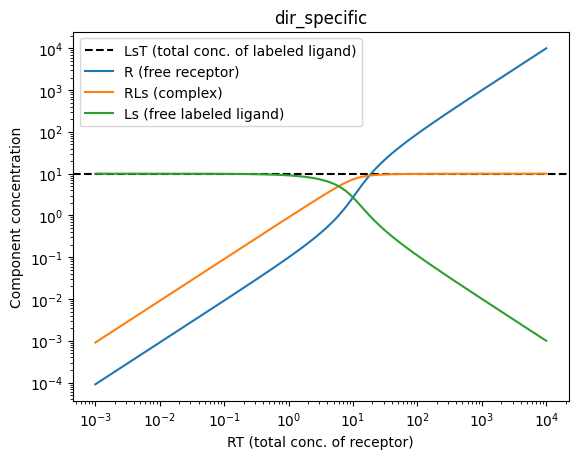
In direct binding, it is assumed that a receptor is titrated to a constant concentration of labeled ligand. In other words, RT is titrated while LsT does not change. Thus, we can treat RT as the independent variable, LsT as a constant, and all other components of the system (R, RLs, Ls) as dependent variables. Here, we will use the dir_specific model to plot the situation. You can play around with the values of LsT and Kds to see how the predicted equilibrium in the system changes.
# Define minimum and maximum
ymin = 0
ymax = 1

# Define experimental constants
LsT = 10       # Total concentration of labeled ligand
Kds = 1        # Kd of labeled ligand

# Get a range of values for the titrated component
RT = np.logspace(np.log10(0.001), np.log10(10000), 1000)

# Call the model and get concentrations of the system components
model, R, RLs, Ls = bc.dir_specific(RT, ymin, ymax, LsT, Kds)

# Plot LsT as horizontal line (it is constant during experiment)
plt.axhline(y = LsT, linestyle="--", color="black", label="LsT (total conc. of labeled ligand)")

# Plot concentrations of the system components
plt.plot(RT, R, label="R (free receptor)")
plt.plot(RT, RLs, label="RLs (complex)")
plt.plot(RT, Ls, label="Ls (free labeled ligand)")

# Set up and show the plot
plt.title("dir_specific")
plt.xlabel("RT (total conc. of receptor)")
plt.ylabel("Component concentration")
plt.xscale("log")
plt.yscale("log")
plt.legend()
plt.show()
Competitive binding
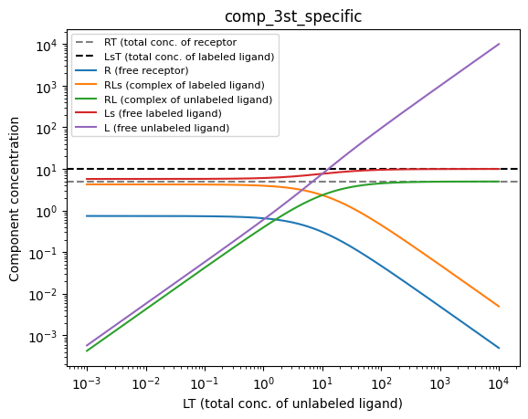
In competitive binding, it is assumed that the unlabeled ligand is titrated to a constant concentration of receptor and labeled ligand. In other words, LT is titrated while RT and LsT do not change. Thus, we can treat LT as the independent variable, RT and LsT as constants, and all other components of the system (R, RLs, RL, Ls, L) as dependent variables. Here, we will use the comp_3st_specific model to plot the situation. You can play around with the values of RT, LsT, Kds and Kd to see how the predicted equilibrium in the system changes.
# Define minimum and maximum
ymin = 0
ymax = 1

# Define experimental constants
RT = 5         # Total concentration of receptor
LsT = 10       # Total concentration of labeled ligand
Kds = 1        # Kd of labeled ligand
Kd = 1         # Kd of unlabeled ligand

# Get a range of values for the titrated component
LT = np.logspace(np.log10(0.001), np.log10(10000), 1000)

# Call the model and get concentrations of the system components
model, R, RLs, RL, Ls, L = bc.comp_3st_specific(LT, ymin, ymax, RT, LsT, Kds, Kd)

# Plot LsT as horizontal line (it is constant during experiment)
plt.axhline(y = RT, linestyle="--", color="grey", label="RT (total conc. of receptor")
plt.axhline(y = LsT, linestyle="--", color="black", label="LsT (total conc. of labeled ligand)")

# Plot concentrations of the system components
plt.plot(LT, R, label="R (free receptor)")
plt.plot(LT, RLs, label="RLs (complex of labeled ligand)")
plt.plot(LT, RL, label="RL (complex of unlabeled ligand)")
plt.plot(LT, Ls, label="Ls (free labeled ligand)")
plt.plot(LT, L, label="L (free unlabeled ligand)")

# Set up and show the plot
plt.title("comp_3st_specific")
plt.xlabel("LT (total conc. of unlabeled ligand)")
plt.ylabel("Component concentration")
plt.xscale("log")
plt.yscale("log")
plt.legend(fontsize = 8)
plt.show()