Competitive-binding Kd

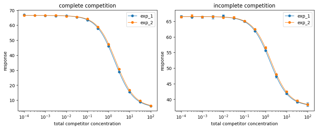
This tutorial fits complete three-state and incomplete four-state competition. Both examples use total competitor concentration on the x-axis. Review the equilibrium model assumptions before interpreting the fitted Kd values.

import matplotlib.pyplot as plt

import bindcurve as bc

all_data = bc.DoseResponseData.from_csv(
    "data/competitive-binding.csv",
    format="wide",
)
data = all_data.keep_only(["three_state", "four_state"])
data.summary()

	compound_id	N_exp	N_obs	N_conc_total	concentration_min	concentration_max	response_min	response_max
0	four_state	2	78	13	0.0001	100.0	37.69860	67.2401
1	three_state	2	78	13	0.0001	100.0	6.00648	67.1762

Complete three-state competition

Tracer and competitor are mutually exclusive. The total receptor RT, total tracer LsT, and tracer dissociation constant Kds are fixed assay constants.

three_state_data = data.keep_only("three_state")
three_state_results = bc.fit(
    three_state_data,
    model="comp_3st_specific",
    fixed={"RT": 0.05, "LsT": 0.01, "Kds": 0.02},
)
three_state_results.summary()[["compound_id", "N_exp", "Kd"]]

	compound_id	N_exp	Kd
0	three_state	2	0.597135

Incomplete four-state competition

The four-state model permits a ternary complex and additionally requires Kd3, the tracer affinity for competitor-bound receptor.

four_state_data = data.keep_only("four_state")
four_state_results = bc.fit(
    four_state_data,
    model="comp_4st_specific",
    fixed={"RT": 0.05, "LsT": 0.01, "Kds": 0.02, "Kd3": 0.08},
)
four_state_results.summary()[["compound_id", "N_exp", "Kd"]]

	compound_id	N_exp	Kd
0	four_state	2	0.810093

fig, axes = plt.subplots(1, 2, figsize=(10, 4), constrained_layout=True)
bc.plot_fits(three_state_data, three_state_results, ax=axes[0])
bc.plot_fits(four_state_data, four_state_results, ax=axes[1])
axes[0].set_title("complete competition")
axes[1].set_title("incomplete competition")
for ax in axes:
    ax.set_xlabel("total competitor concentration")
    ax.set_ylabel("response")
    ax.legend()
plt.show()

Convert an IC₅₀ to Kd

When only an IC₅₀ is available, the finite-concentration Coleska conversion uses the same complete one-site equilibrium assumptions. The synthetic value below is consistent with Kd = 0.60. See the conversion theory for applicability and alternatives.

bc.convert_ic50_to_kd(
    model="coleska",
    IC50=2.1286835665,
    RT=0.05,
    LsT=0.01,
    Kds=0.02,
)

IC50ConversionResult(compound_id=None, model='coleska', IC50=2.1286835665, Kd=0.5999999999931291, lower_IC50=None, upper_IC50=None, lower_Kd=None, upper_Kd=None)

The comp_3st_total and comp_4st_total variants add the fixed nonspecific competitor factor N; their fitting workflow is otherwise the same.