IC₅₀ analysis

This tutorial fits two synthetic inhibitory dose-response datasets. Each compound has two independent experiments and three technical replicates per concentration. Concentrations are unit-agnostic but use one consistent scale. See the logistic-model theory for the model definition.

import matplotlib.pyplot as plt

import bindcurve as bc

Load the observations

Wide input stores technical replicates in separate response columns. DoseResponseData converts them to the canonical long-form representation.

all_data = bc.DoseResponseData.from_csv(
    "data/competitive-binding.csv",
    format="wide",
)
data = all_data.keep_only(["ic50_a", "ic50_b"])
data.summary()

	compound_id	N_exp	N_obs	N_conc_total	concentration_min	concentration_max	response_min	response_max
0	ic50_a	2	78	13	0.0001	100.0	4.60059	95.2736
1	ic50_b	2	78	13	0.0001	100.0	4.59961	95.3107

Fit and summarize

bindcurve averages technical replicates at each concentration, fits each independent experiment separately, and then summarizes the fitted parameters across experiments. Here the known lower and upper response plateaus are fixed so the fit focuses on IC₅₀ and Hill slope.

results = bc.fit(
    data,
    model="ic50",
    fixed={"ymin": 5.0, "ymax": 95.0},
)

results.summary()[
    ["compound_id", "N_exp", "N_fit_successful", "IC50", "hill_slope"]
]

	compound_id	N_exp	N_fit_successful	IC50	hill_slope
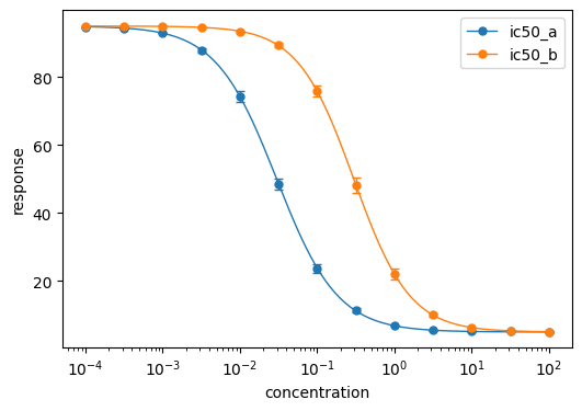
0	ic50_a	2	2	0.029872	1.102240
1	ic50_b	2	2	0.297373	1.200361

results.report(unit="concentration units", include_n_exp=True)

	compound_id	report	N_fit_successful	N_fit_failed
0	ic50_a	0.030 [0.03, 0.03] concentration units, N_exp = 2	2	0
1	ic50_b	0.30 [0.3, 0.3] concentration units, N_exp = 2	2	0

Plot compound summaries

plot_compounds() shows one aggregate series per compound while preserving the experiment-level fits used for the summary.

fig, ax = plt.subplots(figsize=(6, 4))
bc.plot_compounds(data, results, ax=ax)
ax.set_xlabel("concentration")
ax.set_ylabel("response")
ax.legend()
plt.show()