Direct-binding Kd

This tutorial fits the three direct-binding models to purpose-built synthetic compounds. The models differ in their treatment of ligand depletion and nonspecific tracer immobilization; see the equilibrium-binding theory before applying them to experimental data.

import matplotlib.pyplot as plt

import bindcurve as bc

data = bc.DoseResponseData.from_csv(
    "data/direct-binding.csv",
    format="wide",
)
data.summary()

	compound_id	N_exp	N_obs	N_conc_total	concentration_min	concentration_max	response_min	response_max
0	simple	2	72	12	0.001	31.6228	5.07037	94.8318
1	specific	2	72	12	0.001	31.6228	5.16027	95.2123
2	total	2	72	12	0.001	31.6228	4.58529	94.5178

Simple binding

dir_simple treats the concentration axis as free receptor and does not require additional assay constants.

simple_data = data.keep_only("simple")
simple_results = bc.fit(simple_data, model="dir_simple")
simple_results.summary()[["compound_id", "N_exp", "Kds"]]

	compound_id	N_exp	Kds
0	simple	2	0.149727

Depletion-aware binding

dir_specific uses total receptor on the concentration axis and requires the total tracer concentration LsT.

specific_data = data.keep_only("specific")
specific_results = bc.fit(
    specific_data,
    model="dir_specific",
    fixed={"LsT": 0.05},
)
specific_results.summary()[["compound_id", "N_exp", "Kds"]]

	compound_id	N_exp	Kds
0	specific	2	0.199044

Binding with a nonspecific tracer term

dir_total additionally requires the dimensionless nonspecific factor Ns.

total_data = data.keep_only("total")
total_results = bc.fit(
    total_data,
    model="dir_total",
    fixed={"LsT": 0.05, "Ns": 0.30},
)
total_results.summary()[["compound_id", "N_exp", "Kds"]]

	compound_id	N_exp	Kds
0	total	2	0.250722

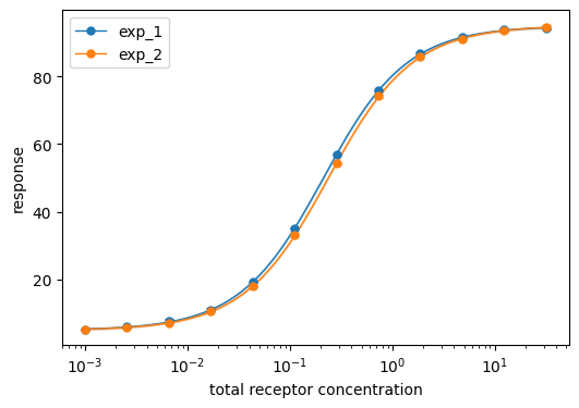
Inspect a representative fit

fig, ax = plt.subplots(figsize=(6, 4))
bc.plot_fits(specific_data, specific_results, ax=ax, confidence_band=True)
ax.set_xlabel("total receptor concentration")
ax.set_ylabel("response")
ax.legend()
plt.show()